The CNN

The Feed Forward neural network is composed of fully connected neurons at each layer, the input is a flattened vector that is feed to the input neurons the network then is restricted from an information point of view .

Because pictures are composed of hiearchies, an image only provides full information if seen in it’s 2D view (3D actually) add to that the fact that colored images introduce a third dimension (color channel) that encodes more information , it will soon become evident that it’s infeasible to scale simple FFN to this task we need a new way to extract features .

CNNs learns a spatial hiearchy of their input a first convolutional layer will learn to detect edges a second will learn larger patterns made of the first one and so … these patterns are also translationally invariant meaning that if they learn a pattern at the top right of a picture they can recognize anywhere else .

The CNN here adds a new trick (patches) also called filters , neurons are not connected to all other neurons but only to a few , each group is then locally connected and learn a partial information about the input map .

===========================================

Feature Maps and Convolutional Layers

These patches become more task-oriented than generalized .

Let’s take a CIFAR-10 sample an image from CIFAR is of size 32x32x3 (width,height,depth) a first convolutional layer will take a 5x5x3 window and slide it across the image a convolution operates on 3D tensors ,feature maps, in CIFAR the depth is 3 (RGB) in mnist because the color is only shades of grey the depth is 1 . The height and width are parameters but the depth is always equal to the image depth .

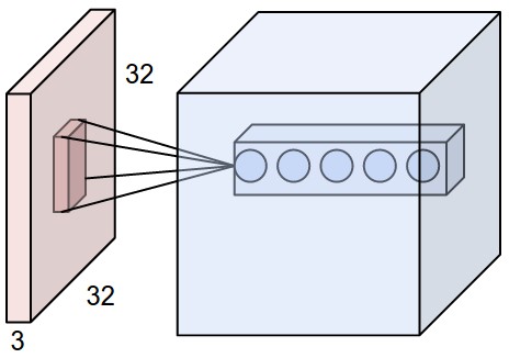
The window or patch will extract a 2D map of the input that encodes certain information ,the output of the patches will be multiplied ( dot product) by a Kernel a transformed patch ( column vector) of the output feature map .

The output of the patches is controlled by 3 parameters depth,stride and padding :

• Depth is the number of filters we would like to use

• Stride is by how many pixels we slide (1 pixel,2 pixel …) we usually use 1 or 2 rarely more than 3

• Padding is just adding zeros to make the size of the input and output balanced

  The Krizhevsky et al. architecture used 11 filters 4 strides and no padding it’s input was of 227x227x3 . The output of this layer had a 55x55x96 size the trick to compute it is Input-Filter/Stride+1 (the architecutre used a layer with a depth = 96

A Python example of what a convolutional layer is like :

• suppose we have an input image of size 11x11x4 and we will use a filter of size 5 the depth of the filter is the same as the input is 4 . let’s compute the output layers (feature map)

    # the first transformed patch (column vector of the output)
    v[0,0,0] = np.sum(X[:5,:5,:] * Ker) 
    v[1,0,0] = np.sum(X[2:7,:5,:] * Ker)
    v[2,0,0] = np.sum(X[4:9,:5,:] *Ker)
    v[3,0,0] = np.sum(X[6:11,:5,:] *Ker)

This is just the first feature map notice how the stride is added to the first component only since we slide in a linear direction .

Max Pooling

The pooling layer always (by practice) follows a convolutional layer to reduce the spatial size of the feature maps to have less parameters to learn . A Pooling layer can be resumed in the following function :

    def max_pool(width,height,depth):
        f = 2 # filter 2 is the most used value in practice
        s = 2 # stride
        
        w = (width - f)/s+1
        h = (height -f)/s+1
        d = depth
        return w*h*d

That’s all so if I had a 32x32x4 output after pooling I will have a 16x16x4 downsampled output twice less parameters to learn .

Practical

In practice you rarely train a CNN from zero usually we leverage transfer-learning to train big networks such as Inception v3 ,VGG16 … and retrain their output layers on our problem classes .

But let’s see what a CNN looks like in Pytorch and Keras :

================================================================

PyTorch :

import torch
from torch.autograd import Variable
import torch.nn as nn
import torch.nn.functional as F


class Net(nn.Module):

    def __init__(self):
        super(Net, self).__init__()
        # 3 input image channel, 6 output channels, 5x5 square convolution
        # kernel
        self.conv1 = nn.Conv2d(3, 6, 5)
        self.conv2 = nn.Conv2d(6, 16, 5)
        # an affine operation: y = Wx + b
        self.fc1 = nn.Linear(16 * 5 * 5, 120)
        self.fc2 = nn.Linear(120, 84)
        self.fc3 = nn.Linear(84, 10)

    def forward(self, x):
        # Max pooling over a (2, 2) window
        x = F.max_pool2d(F.relu(self.conv1(x)), (2, 2))
        # If the size is a square you can only specify a single number
        x = F.max_pool2d(F.relu(self.conv2(x)), 2)
        x = x.view(-1, self.num_flat_features(x))
        x = F.relu(self.fc1(x))
        x = F.relu(self.fc2(x))
        x = self.fc3(x)
        return x

Keras :

# let's build a small convnet for binary classification
from keras import layers,models

model = models.Sequential()

# input is 150,150,3 3 is the depth axis in the case of RGB it's 3 for each color channel red,green,blue
model.add(layers.Conv2D(32,(3,3),activation='relu',input_shape=(150,150,3)))
model.add(layers.MaxPooling2D((2,2)))

model.add(layers.Conv2D(64,(3,3),activation='relu'))
model.add(layers.MaxPooling2D((2,2)))

model.add(layers.Conv2D(128,(3,3),activation='relu'))
model.add(layers.MaxPooling2D((2,2)))

model.add(layers.Conv2D(128,(3,3),activation='relu'))
model.add(layers.MaxPooling2D((2,2)))
#flatten and fc layer 
model.add(layers.Flatten())
model.add(layers.Dense(512,activation='relu'))
#output 1 neuron activated using sigmoid for b-class task
model.add(layers.Dense(1,activation='sigmoid'))

N.B :

• ressources :

  • Chapter 5,Deep Learning in Python by F.Chollet
  • CS231n.github.io

• implementation:

  • Notebook